Monte Carlo Simulation Methodology

Why a Single Projection Is Not Enough

Most retirement calculators show you one number: "If your investments return 7% per year, you will have $X at age 65." That number is built on an assumption that never happens in real life. Markets do not return a steady 7% every year. They return 22% one year, negative 15% the next, 8% the year after that.

The order in which those returns arrive matters enormously, especially during retirement. If you retire and immediately experience two or three bad years while withdrawing money to live on, your portfolio takes a hit it may never recover from. This is called sequence-of-returns risk, and it is the single biggest threat to a retirement plan that looks fine on paper.

Monte Carlo simulation addresses this problem directly. Instead of showing you one future, it shows you thousands of possible futures, each with a different random sequence of market returns. The result is not a single number but a probability: "Given your plan, your money lasts in 85% of the scenarios we tested."

That probability is far more useful than any single projection because it accounts for the uncertainty that every retiree actually faces.

How RetirePlanAI's Monte Carlo Engine Works

Here is a step-by-step explanation of what happens when you run a Monte Carlo simulation in RetirePlanAI.

The Simulation Parameters

RetirePlanAI runs 5,000 independent simulations. This is sufficient for reliable probability estimates in nearly all cases.

Each simulation covers your entire retirement period, from your planned retirement age through your life expectancy (age 95). If you plan to retire at 62 and plan through age 95, each simulation models 33 years of annual market returns, withdrawals, income, expenses, and taxes.

The Return Model: Log-Normal Distribution

RetirePlanAI uses a log-normal distribution to generate random market returns. This is an important technical choice, and it is worth understanding why.

A normal distribution (the classic bell curve) would imply that positive and negative returns are equally likely and that there is no limit to how negative a return can be. In reality, the worst a market can do in a single year is lose 100% (you cannot lose more than everything), and markets historically show a slight positive skew, meaning large positive years are somewhat more likely than equivalently large negative years.

The log-normal distribution captures these real-world properties. It ensures that returns cannot go below negative 100%, and it produces the asymmetric distribution that matches how actual stock and bond markets have behaved historically. This means the simulated futures reflect realistic market behavior, not a simplified mathematical convenience.

The distribution is parameterized using the expected return and standard deviation (volatility) from your plan assumptions. If you set an expected stock return of 10% with a standard deviation of 15%, the simulation generates random returns that cluster around 10% but can swing significantly in any given year, following the log-normal shape.

The Two-Bucket Portfolio Model

RetirePlanAI divides your accounts into two categories that behave differently in the simulation:

• Market accounts: Stocks, bonds, mutual funds, ETFs, and any investment subject to market volatility. These accounts experience the randomized returns generated by the Monte Carlo engine. In each simulation, each year, these accounts get a different return drawn from the log-normal distribution.
• Stable accounts: Cash, CDs, money market funds, stable value funds, and similar low-volatility holdings. These accounts grow at the rate of return you configured for each account. They are not subject to the randomized market returns because their real-world behavior is predictable and low-variance.

This two-bucket approach matters because a portfolio that is 70% stocks and 30% cash behaves very differently from a portfolio that is 100% stocks. The stable bucket provides a buffer against market volatility, and the simulation accurately reflects that buffer.

What Happens in Each Simulation

For each of the 5,000 simulations, the engine walks through every year of your retirement and does the following:

1. Generates a random market return for that year using the log-normal distribution.
2. Applies that return to your market accounts. Applies the stable growth rate to your stable accounts.
3. Adds any income for that year (Social Security, pensions, part-time work, rental income).
4. Subtracts your planned spending for that year (adjusted for any spending changes you have modeled).
5. Subtracts any one-time expenses scheduled for that year.
6. Calculates whether your portfolio balance has reached zero.

If the portfolio reaches zero before the end of the simulation period, that simulation is marked as a failure. If money remains at the end, it is marked as a success.

Understanding the Results

Success Rate

The headline number is the success rate: the percentage of simulations where your money lasted through your entire plan. If 4,250 out of 5,000 simulations succeed, your success rate is 85%.

What does a given success rate mean in practical terms?

• 90% or higher: Your plan is robust. It survives in the vast majority of market conditions, including many bad scenarios. Plans in this range can generally tolerate moderate unexpected expenses or lower-than-expected returns.
• 80-89%: Generally considered acceptable for most planners. Your plan succeeds in most scenarios but has some vulnerability to extended poor market conditions. This range works well for people who have some flexibility to adjust spending if markets underperform.
• 70-79%: A caution zone. Roughly one in four simulated futures fails. If you have flexibility (willing to cut spending, work part-time, or downsize), this may be acceptable. If your spending is relatively fixed, this range suggests adjustments are needed.
• Below 70%: Significant risk of running out of money. At this level, your plan depends on getting reasonably good market conditions to survive. Consider increasing savings, delaying retirement, reducing planned spending, or exploring other adjustments.

There is no universally "right" success rate. A person with a guaranteed pension covering 80% of their expenses can tolerate a lower portfolio success rate than someone relying entirely on portfolio withdrawals. Context matters.

Percentile Outcomes

Beyond the pass/fail success rate, RetirePlanAI reports percentile outcomes that show the range of possible portfolio values:

• 10th percentile: The portfolio value that 90% of simulations exceeded. This represents a near-worst-case scenario. If your 10th percentile at age 90 is $200,000, that means even in a bad-luck scenario, you likely still have $200,000 left.
• Median (50th percentile): The middle outcome. Half of simulations end with more than this value, half with less. This is the most representative "expected" outcome, and it is more reliable than the average because it is not skewed by extreme outcomes.
• 90th percentile: The portfolio value that only 10% of simulations exceeded. This represents a best-case scenario. It is interesting for estate planning, but you should not plan your spending around it.

If your plan fails in some simulations, RetirePlanAI also reports the median depletion age: the age at which money runs out in the median failed simulation. This helps you understand the severity of failure. Running out of money at 94 is a very different situation than running out at 78.

Additional Analysis Tools

Monte Carlo simulation is the foundation, but RetirePlanAI builds several additional tools on top of it.

Sensitivity Analysis

Sensitivity analysis tests which input variables have the biggest impact on your success rate. The tool systematically varies each major assumption (investment returns, inflation, spending level, lifespan) and measures how much your success rate changes.

This is valuable because it tells you where to focus your attention. If your success rate barely changes when you adjust inflation from 3% to 4%, but drops sharply when you increase spending by $5,000, you know that controlling spending is far more important than worrying about inflation for your specific plan.

Market Replay Heatmap (1928-2024)

The market replay tool takes a different approach from Monte Carlo. Instead of generating random returns, it uses actual historical market data. It runs your exact cash flow plan against every possible historical starting year from 1928 through 2024.

The result is a decade-by-decade heatmap that shows how your plan would have fared if you had retired during the Great Depression, during the post-war boom, during the 1970s stagflation, during the dot-com bubble, during the 2008 financial crisis, or during the 2020 pandemic.

This tool answers a different question from Monte Carlo. Monte Carlo asks, "How likely is my plan to succeed given random future markets?" Market replay asks, "Would my plan have survived the worst periods in recorded market history?" Both questions are valuable.

Find Max Safe Withdrawal Rate

This tool uses a binary search algorithm to find the maximum amount you can withdraw annually while still achieving your target success rate. You specify your desired success rate (for example, 85%), and the tool searches for the highest spending level that achieves it.

This directly answers one of the most common retirement planning questions: "What is the most I can safely spend each year?" The answer is personalized to your specific financial situation, including your income sources, account types, tax treatment, and risk tolerance.

Detailed Trajectory Analysis

The detailed trajectory visualization shows your portfolio's range of possible outcomes as percentile bands. These bands represent the 10th, 25th, 50th (median), 75th, and 90th percentiles across all successful simulations, giving you a clear picture of best-case, worst-case, and most likely outcomes at every age.

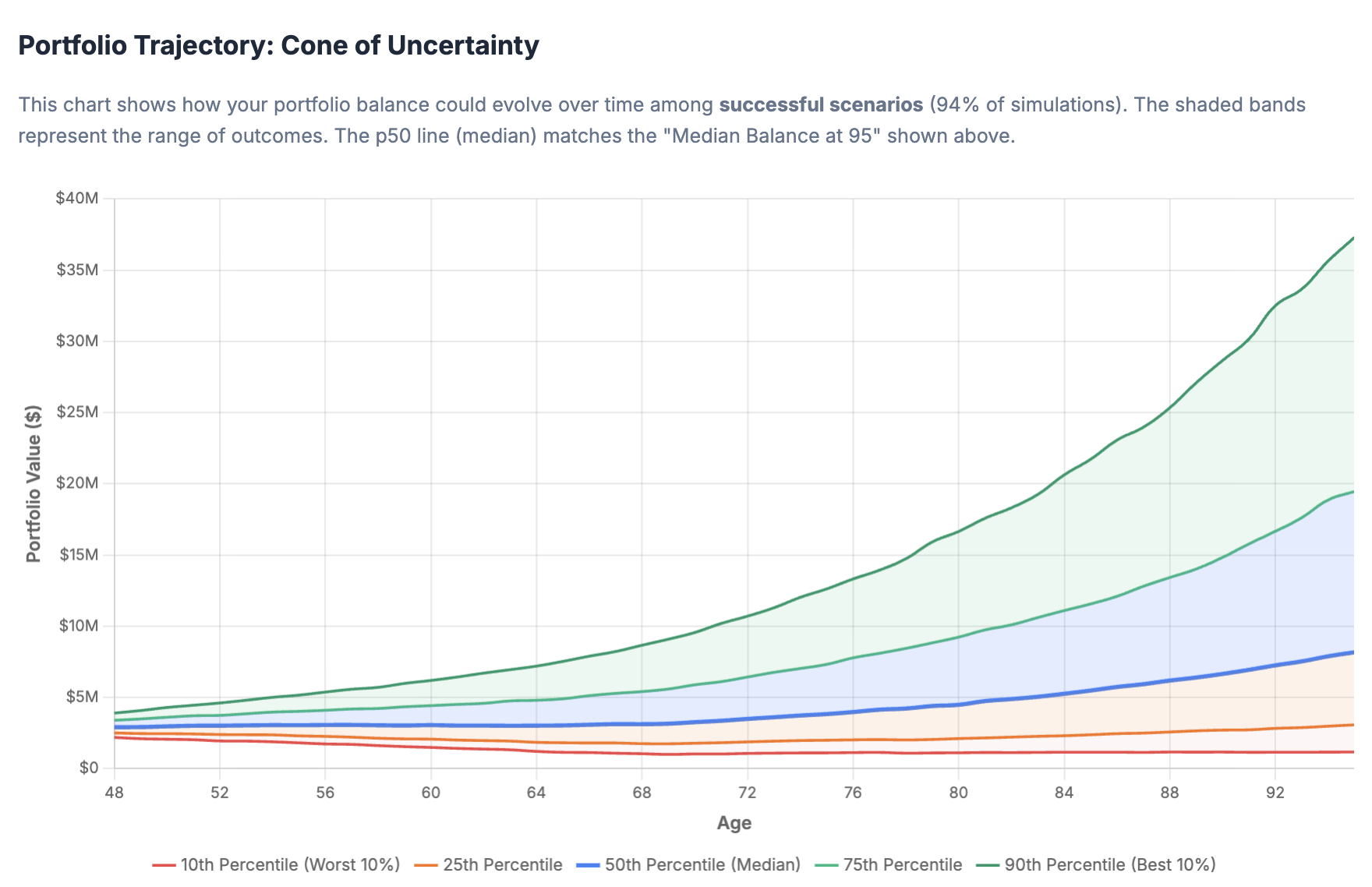
The width of the bands communicates the range of uncertainty. Narrow bands mean most simulations agree on the outcome; wide bands mean there is significant variation depending on market conditions. The median line shows the most typical path, while the outer bands show how far outcomes can diverge.

Tips for Getting the Most from Monte Carlo

• Run it after any significant change to your plan. Updated your spending goal? Changed your retirement age? Added an account? Run Monte Carlo again to see how your success rate changed.
• Pay attention to the 10th percentile, not just the success rate. A 90% success rate where the 10th percentile leaves you with $50,000 at age 90 is very different from a 90% success rate where the 10th percentile leaves you with $500,000. The percentile outcomes tell you about the severity of risk, not just its probability.
• Use sensitivity analysis to prioritize. Do not try to optimize everything at once. Find out which variable matters most for your plan and focus there.
• Do not chase 100%. A 100% success rate means your plan survives even the most extreme market scenarios. That sounds safe, but it also means you are probably spending significantly less than you could. Most planners recommend targeting 80-90% and maintaining flexibility to adjust.
• Compare scenarios, not just individual results. The power of Monte Carlo is in comparing alternatives. "Scenario A has an 82% success rate and scenario B has 91%" is far more actionable than just knowing your single success rate.